arviz_plots.plot_loo_pit#
- arviz_plots.plot_loo_pit(dt, ci_prob=None, coverage=False, var_names=None, filter_vars=None, group='posterior_predictive', coords=None, sample_dims=None, plot_collection=None, backend=None, labeller=None, aes_by_visuals=None, visuals=None, stats=None, **pc_kwargs)[source]#
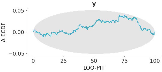
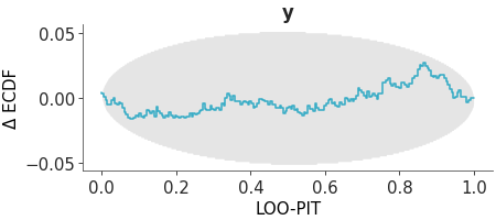
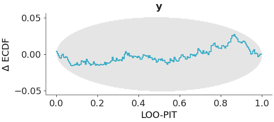
LOO-PIT Δ-ECDF values with simultaneous confidence envelope.
For a calibrated model the LOO Probability Integral Transform (PIT) values, $p(tilde{y}_i le y_i mid y_{-i})$, should be uniformly distributed. Where $y_i$ represents the observed data for index $i$ and $tilde y_i$ represents the posterior predictive sample at index $i$. $y_{-i}$ indicates we have left out the $i$-th observation. LOO-PIT values are computed using the PSIS-LOO-CV method described in [1] and [2].
This plot shows the empirical cumulative distribution function (ECDF) of the LOO-PIT values. To make the plot easier to interpret, we plot the Δ-ECDF, that is, the difference between the observed ECDF and the expected CDF. Simultaneous confidence bands are computed using the method described in described in [3].
Alternatively, we can visualize the coverage of the central posterior credible intervals by setting
coverage=True. This allows us to assess whether the credible intervals includes the observed values. We can obtain the coverage of the central intervals from the LOO-PIT by replacing the LOO-PIT with two times the absolute difference between the LOO-PIT values and 0.5.For more details on how to interpret this plot, see https://arviz-devs.github.io/EABM/Chapters/Prior_posterior_predictive_checks.html#pit-ecdfs.
- Parameters:
- dt
xarray.DataTree Input data
- ci_prob
float, optional Indicates the probability that should be contained within the plotted credible interval. Defaults to
rcParams["stats.ci_prob"]- coveragebool, optional
If True, plot the coverage of the central posterior credible intervals. Defaults to False.
- var_names
strorlistofstr, optional One or more variables to be plotted. Currently only one variable is supported. Prefix the variables by ~ when you want to exclude them from the plot.
- filter_vars{
None, “like”, “regex”}, optional, default=None If None (default), interpret var_names as the real variables names. If “like”, interpret var_names as substrings of the real variables names. If “regex”, interpret var_names as regular expressions on the real variables names.
- coords
dict, optional Coordinates to plot.
- sample_dims
stror sequence of hashable, optional Dimensions to reduce unless mapped to an aesthetic. Defaults to
rcParams["data.sample_dims"]- plot_collection
PlotCollection, optional - backend{“matplotlib”, “bokeh”, “plotly”}, optional
- labeller
labeller, optional - aes_by_visualsmapping of {
strsequence ofstr}, optional Mapping of visuals to aesthetics that should use their mapping in
plot_collectionwhen plotted. Valid keys are the same as forvisuals.- visualsmapping of {
strmapping orFalse}, optional Valid keys are:
ecdf_lines -> passed to
ecdf_linecredible_interval -> passed to
ci_line_yxlabel -> passed to
labelled_xylabel -> passed to
labelled_ytitle -> passed to
labelled_title
- statsmapping, optional
Valid keys are:
ecdf_pit -> passed to
ecdf_pit. Default is{"n_simulation": 1000}.
- **pc_kwargs
Passed to
arviz_plots.PlotCollection.grid
- dt
- Returns:
References
[1]Vehtari et al. Practical Bayesian model evaluation using leave-one-out cross-validation and WAIC. Statistics and Computing. 27(5) (2017) https://doi.org/10.1007/s11222-016-9696-4
[2]Vehtari et al. Pareto Smoothed Importance Sampling. Journal of Machine Learning Research, 25(72) (2024) https://jmlr.org/papers/v25/19-556.html
[3]Säilynoja et al. Graphical test for discrete uniformity and its applications in goodness-of-fit evaluation and multiple sample comparison. Statistics and Computing 32(32). (2022) https://doi.org/10.1007/s11222-022-10090-6
Examples
Plot the ecdf-PIT for the crabs hurdle-negative-binomial dataset.
>>> from arviz_plots import plot_loo_pit, style
>>> style.use("arviz-variat")
>>> from arviz_base import load_arviz_data
>>> dt = load_arviz_data('radon')
>>> plot_loo_pit(dt)
Plot the coverage for the crabs hurdle-negative-binomial dataset.
>>> plot_loo_pit(dt, coverage=True)