arviz_plots.plot_energy

arviz_plots.plot_energy(dt, bfmi=False, kind=None, plot_collection=None, backend=None, labeller=None, aes_by_visuals=None, visuals=None, stats=None, **pc_kwargs)

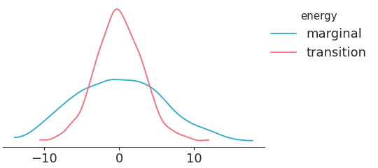
Plot transition distribution and marginal energy distribution in HMC algorithms.

This may help to diagnose poor exploration by gradient-based algorithms like HMC or NUTS. The energy function in HMC can identify posteriors with heavy tailed distributions, that in practice are challenging for sampling.

This plot is in the style of the one used in [1].

Parameters:

dtxarray.DataTree

sample_stats group with an energy variable is mandatory.

bfmibool

Whether to the plot the value of the estimated Bayesian fraction of missing information. Defaults to False. Not implemented yet.

kind{“kde”, “hist”, “dot”, “ecdf”}, optional

How to represent the marginal density. Defaults to rcParams["plot.density_kind"]

plot_collectionPlotCollection, optional

backend{“matplotlib”, “bokeh”, “plotly”}, optional

labellerlabeller, optional

aes_by_visualsmapping of {strsequence of str}, optional

Mapping of visuals to aesthetics that should use their mapping in plot_collection when plotted. Valid keys are the same as for visuals.

visualsmapping of {strmapping or False}, optional

Valid keys are:

• dist -> depending on the value of kind passed to:

  • “kde” -> passed to line_xy

  • “ecdf” -> passed to ecdf_line

  • “hist” -> passed to :func: hist

• title -> passed to labelled_title

• legend -> passed to arviz_plots.PlotCollection.add_legend

• remove_axis -> not passed anywhere, can only be False to skip calling this function

statsmapping, optional

Valid keys are:

• dist -> passed to kde, ecdf, …

**pc_kwargs

Passed to arviz_plots.PlotCollection.wrap

Returns:

PlotCollection

References

[1]

Betancourt. Diagnosing Suboptimal Cotangent Disintegrations in Hamiltonian Monte Carlo. (2016) https://arxiv.org/abs/1604.00695

Examples

Plot a default energy plot

>>> from arviz_plots import plot_energy, style
>>> style.use("arviz-variat")
>>> from arviz_base import load_arviz_data
>>> schools = load_arviz_data('centered_eight')
>>> plot_energy(schools)

Plot transition and marginal energy distributions

Energy

Energy