arviz_plots.plot_dist#
- arviz_plots.plot_dist(dt, var_names=None, filter_vars=None, group='posterior', coords=None, sample_dims=None, kind=None, point_estimate=None, ci_kind=None, ci_prob=None, plot_collection=None, backend=None, labeller=None, aes_by_visuals=None, visuals=None, stats=None, **pc_kwargs)[source]#
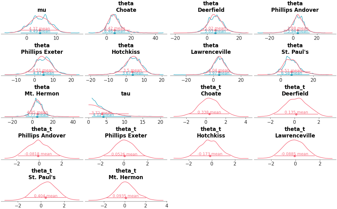
Plot 1D marginal densities in the style of John K. Kruschke’s book [1].
Generate faceted plots with: a graphical representation of 1D marginal densities (as KDE, histogram, ECDF or dotplot), a credible interval and a point estimate.
- Parameters:
- dt
xarray.DataTreeordictof {strxarray.DataTree} Input data. In case of dictionary input, the keys are taken to be model names. In such cases, a dimension “model” is generated and can be used to map to aesthetics.
- var_names
strorlistofstr, optional One or more variables to be plotted. Prefix the variables by ~ when you want to exclude them from the plot.
- filter_vars{
None, “like”, “regex”}, default=None If None, interpret var_names as the real variables names. If “like”, interpret var_names as substrings of the real variables names. If “regex”, interpret var_names as regular expressions on the real variables names.
- group
str, default “posterior” Group to be plotted.
- coords
dict, optional - sample_dims
stror sequence of hashable, optional Dimensions to reduce unless mapped to an aesthetic. Defaults to
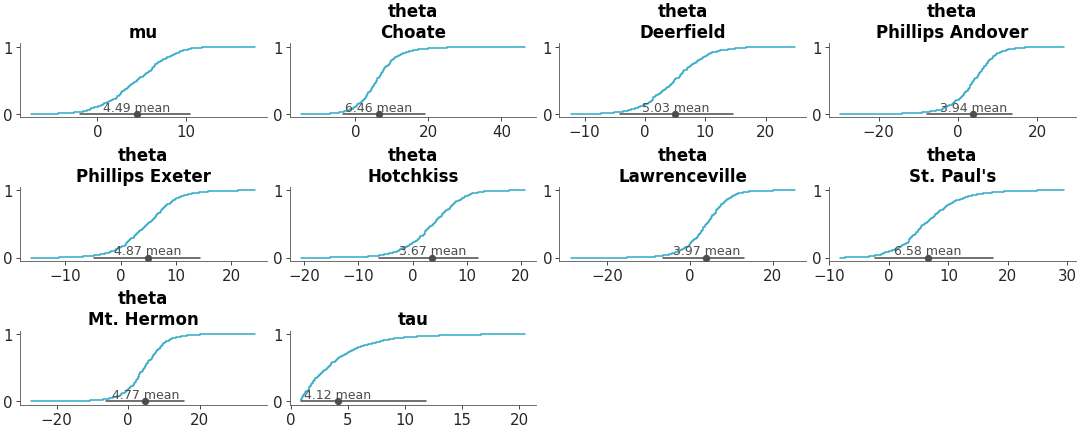
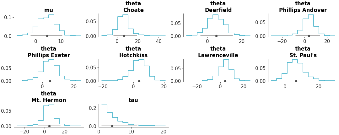
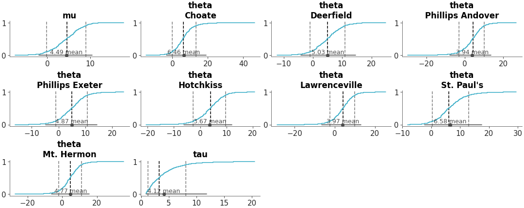
rcParams["data.sample_dims"]- kind{“kde”, “hist”, “dot”, “ecdf”}, optional
How to represent the marginal density. Defaults to
rcParams["plot.density_kind"]- point_estimate{“mean”, “median”, “mode”}, optional
Which point estimate to plot. Defaults to rcParam
stats.point_estimate- ci_kind{“eti”, “hdi”}, optional
Which credible interval to use. Defaults to
rcParams["stats.ci_kind"]- ci_prob
float, optional Indicates the probability that should be contained within the plotted credible interval. Defaults to
rcParams["stats.ci_prob"]- plot_collection
PlotCollection, optional - backend{“matplotlib”, “bokeh”}, optional
- labeller
labeller, optional - aes_by_visualsmapping of {
strsequence ofstr}, optional Mapping of visuals to aesthetics that should use their mapping in
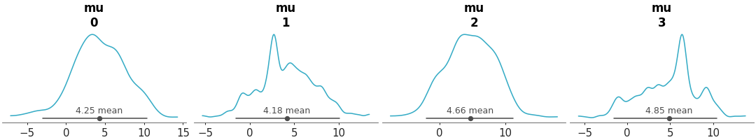
plot_collectionwhen plotted. Valid keys are the same as forvisuals.With a single model, no aesthetic mappings are generated by default, each variable+coord combination gets a plot but they all look the same, unless there are user provided aesthetic mappings. With multiple models,
plot_distmaps “color” and “y” to the “model” dimension.By default, all aesthetics but “y” are mapped to the density representation, and if multiple models are present, “color” and “y” are mapped to the credible interval and the point estimate.
When “point_estimate” key is provided but “point_estimate_text” isn’t, the values assigned to the first are also used for the second.
- visualsmapping of {
strmapping orFalse}, optional Valid keys are:
dist -> depending on the value of kind passed to:
face -> visual that fills the area under the marginal distribution representation.
Defaults to False. Depending on the value of kind it is passed to:
“kde” or “ecdf” -> passed to
fill_between_y“hist” -> passed to
hist
credible_interval -> passed to
line_xpoint_estimate -> passed to
scatter_xpoint_estimate_text -> passed to
point_estimate_texttitle -> passed to
labelled_titlerug -> passed to
scatter_x. Defaults to False.remove_axis -> not passed anywhere, can only be
Falseto skip calling this function
- statsmapping, optional
Valid keys are:
dist -> passed to kde, ecdf, …
credible_interval -> passed to eti or hdi
point_estimate -> passed to mean, median or mode
- **pc_kwargs
Passed to
arviz_plots.PlotCollection.wrap
- dt
- Returns:
See also
- Introduction to batteries-included plots
General introduction to batteries-included plotting functions, common use and logic overview
References
[1]Kruschke. Doing Bayesian Data Analysis, Second Edition: A Tutorial with R, JAGS, and Stan. Academic Press, 2014. ISBN 978-0-12-405888-0. https://www.sciencedirect.com/book/9780124058880
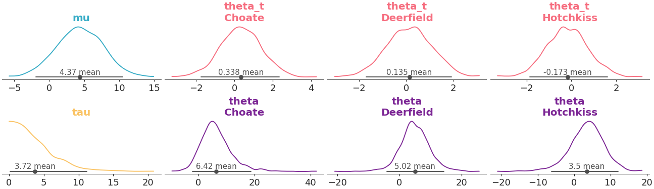
Examples
Map the color to the variable, and have the mapping apply to the title too instead of only the density representation:
>>> from arviz_plots import plot_dist, style
>>> style.use("arviz-variat")
>>> from arviz_base import load_arviz_data
>>> non_centered = load_arviz_data('non_centered_eight')
>>> pc = plot_dist(
>>>     non_centered,
>>>     coords={"school": ["Choate", "Deerfield", "Hotchkiss"]},
>>>     aes={"color": ["__variable__"]},
>>>     aes_by_visuals={"title": ["color"]},
>>> )