arviz_plots.plot_psense_dist#
- arviz_plots.plot_psense_dist(dt, alphas=None, var_names=None, filter_vars=None, prior_var_names=None, likelihood_var_names=None, prior_coords=None, likelihood_coords=None, coords=None, sample_dims=None, kind=None, point_estimate=None, ci_kind=None, ci_prob=None, plot_collection=None, backend=None, labeller=None, aes_by_visuals=None, visuals=None, stats=None, **pc_kwargs)[source]#
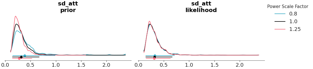
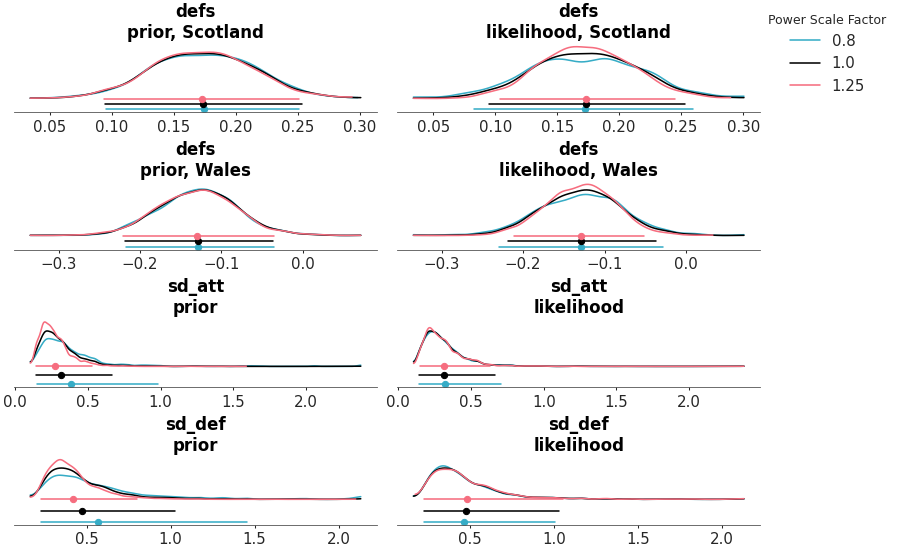
Plot power scaled posteriors.
The posterior sensitivity is assessed by power-scaling the prior or likelihood and visualizing the resulting changes, using Pareto-smoothed importance sampling to avoid refitting as explained in [1].
- Parameters:
- dt
xarray.DataTree Input data
- alphas
tupleoffloat Lower and upper alpha values for power scaling. Defaults to (0.8, 1.25).
- var_names
strorlistofstr, optional One or more variables to be plotted. Prefix the variables by ~ when you want to exclude them from the plot.
- filter_vars{
None, “like”, “regex”}, optional, default=None If None (default), interpret var_names as the real variables names. If “like”, interpret var_names as substrings of the real variables names. If “regex”, interpret var_names as regular expressions on the real variables names.
- prior_var_names
str, optional Name of the log-prior variables to include in the power scaling sensitivity diagnostic
- likelihood_var_names
str, optional Name of the log-likelihood variables to include in the power scaling sensitivity diagnostic
- prior_coords
dict, optional Coordinates defining a subset over the group element for which to compute the log-prior sensitivity diagnostic
- likelihood_coords
dict, optional Coordinates defining a subset over the group element for which to compute the log-likelihood sensitivity diagnostic
- coords
dict, optional - sample_dims
stror sequence of hashable, optional Dimensions to reduce unless mapped to an aesthetic. Defaults to
rcParams["data.sample_dims"]- kind{“kde”, “hist”, “dot”, “ecdf”}, optional
How to represent the marginal distribution.
- point_estimate{“mean”, “median”, “mode”}, optional
Which point estimate to plot. Defaults to rcParam
stats.point_estimate- ci_kind{“eti”, “hdi”}, optional
Which credible interval to use. Defaults to
rcParams["stats.ci_kind"]- ci_prob
float, optional Indicates the probability that should be contained within the plotted credible interval. Defaults to
rcParams["stats.ci_prob"]- plot_collection
PlotCollection, optional - backend{“matplotlib”, “bokeh”, “plotly”}, optional
- labeller
labeller, optional - aes_by_visualsmapping of {
strsequence ofstr}, optional Mapping of visuals to aesthetics that should use their mapping in
plot_collectionwhen plotted. Valid keys are the same as forvisualsexcept for “remove_axis”- visualsmapping of {
strmapping orFalse}, optional Valid keys are:
dist -> depending on the value of kind passed to:
credible_interval -> passed to
line_xpoint_estimate -> passed to
scatter_xpoint_estimate_text -> passed to
point_estimate_texttitle -> passed to
labelled_titlelegend -> passed to
arviz_plots.PlotCollection.add_legendremove_axis -> not passed anywhere, can only be
Falseto skip calling this function
- statsmapping, optional
Valid keys are:
dist -> passed to kde, ecdf, …
credible_interval -> passed to eti or hdi
point_estimate -> passed to mean, median or mode
- **pc_kwargs
Passed to
arviz_plots.PlotCollection.wrap
- dt
- Returns:
References
[1]Kallioinen et al, Detecting and diagnosing prior and likelihood sensitivity with power-scaling, Stat Comput 34, 57 (2024), https://doi.org/10.1007/s11222-023-10366-5
Examples
Select a single variable and generate a point-interval plot
>>> from arviz_plots import plot_psense_dist, style
>>> style.use("arviz-variat")
>>> from arviz_base import load_arviz_data
>>> rugby = load_arviz_data('rugby')
>>> plot_psense_dist(rugby, var_names=["sd_att"], visuals={"kde":False})