arviz_plots.plot_ess#
- arviz_plots.plot_ess(dt, var_names=None, filter_vars=None, group='posterior', coords=None, sample_dims=None, kind='local', relative=False, rug=False, rug_kind='diverging', n_points=20, extra_methods=False, min_ess=400, plot_collection=None, backend=None, labeller=None, aes_by_visuals=None, visuals=None, stats=None, **pc_kwargs)[source]#
Plot effective sample size plots.
Roughly speaking, the effective sample size of a quantity of interest captures how many independent draws contain the same amount of information as the dependent sample obtained by the MCMC algorithm. The higher the ESS the better. See [1] for more details.
- Parameters:
- dt
xarray.DataTreeordictof {strxarray.DataTree} Input data. In case of dictionary input, the keys are taken to be model names. In such cases, a dimension “model” is generated and can be used to map to aesthetics.
- var_names
stror sequence ofstr, optional One or more variables to be plotted. Prefix the variables by ~ when you want to exclude them from the plot.
- filter_vars{
None, “like”, “regex”}, defaultNone If None, interpret var_names as the real variables names. If “like”, interpret var_names as substrings of the real variables names. If “regex”, interpret var_names as regular expressions on the real variables names.
- group
str, default “posterior” Group to be plotted.
- coords
dict, optional - sample_dims
stror sequence of hashable, optional Dimensions to reduce unless mapped to an aesthetic. Defaults to
rcParams["data.sample_dims"]- kind{“local”, “quantile”}, default “local”
Specify the kind of plot:
The
kind="local"argument generates the ESS’ local efficiency for estimating small-interval probability of a desired posterior.The
kind="quantile"argument generates the ESS’ local efficiency for estimating quantiles of a desired posterior.
- relativebool, default
False Show relative ess in plot
ress = ess / N.- rugbool, default
False Add a rug plot for a specific subset of values.
- rug_kind
str, default “diverging” Variable in sample stats to use as rug mask. Must be a boolean variable.
- n_points
int, default 20 Number of points for which to plot their quantile/local ess or number of subsets in the evolution plot.
- extra_methodsbool, default
False Plot mean and sd ESS as horizontal lines.
- min_ess
int, default 400 Minimum number of ESS desired. If
relative=Truethe line is plotted atmin_ess / n_samplesfor local and quantile kinds- plot_collection
PlotCollection, optional - backend{“matplotlib”, “bokeh”}, optional
- labeller
labeller, optional - aes_by_visualsmapping of {
strsequence ofstrorFalse}, optional Mapping of visuals to aesthetics that should use their mapping in
plot_collectionwhen plotted. Valid keys are the same as forvisuals.By default, no aesthetic mappings are defined. Only when multiple models are present a color and x shift is generated to distinguish the data coming from the different models.
When
meanorsdkeys are present in aes_by_visuals butmean_textorsd_textare not, the respective_textkey will be added with the same values asmeanorsdones.- visualsmapping of {
strmapping orFalse}, optional Valid keys are:
ess -> passed to
scatter_xyrug -> passed to
trace_rugmean -> passed to
line_xymean_text -> passed to
annotate_xysd_text -> passed to
annotate_xysd -> passed to
line_xymin_ess -> passed to
line_xytitle -> passed to
labelled_titlexlabel -> passed to
labelled_xylabel -> passed to
labelled_ylegend -> passed to
arviz_plots.PlotCollection.add_legend
- statsmapping, optional
Valid keys are:
ess -> passed to ess, method = ‘local’ or ‘quantile’ based on kind
mean -> passed to ess, method=’mean’
sd -> passed to ess, method=’sd’
- **pc_kwargs
Passed to
arviz_plots.PlotCollection.wrap
- dt
- Returns:
See also
- Introduction to batteries-included plots
General introduction to batteries-included plotting functions, common use and logic overview
References
[1]Vehtari et al. Rank-normalization, folding, and localization: An improved Rhat for assessing convergence of MCMC. Bayesian Analysis. 16(2) (2021) https://doi.org/10.1214/20-BA1221. arXiv preprint https://arxiv.org/abs/1903.08008
Examples
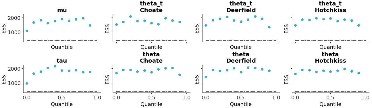
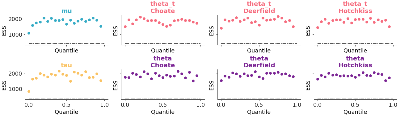
We can manually map the color to the variable, and have the mapping apply to the title too instead of only the ess markers:
>>> from arviz_plots import plot_ess, style
>>> style.use("arviz-variat")
>>> from arviz_base import load_arviz_data
>>> non_centered = load_arviz_data('non_centered_eight')
>>> pc = plot_ess(
>>>     non_centered,
>>>     coords={"school": ["Choate", "Deerfield", "Hotchkiss"]},
>>>     aes={"color": ["__variable__"]},
>>>     aes_by_visuals={"title": ["color"]},
>>> )
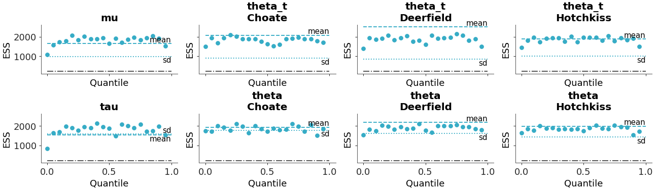
We can add extra methods to plot the mean and standard deviation as lines, and adjust the minimum ess baseline as well:
>>> pc = plot_ess(
>>>     non_centered,
>>>     coords={"school": ["Choate", "Deerfield", "Hotchkiss"]},
>>>     extra_methods=True,
>>>     min_ess=200,
>>> )
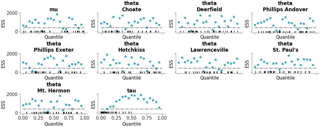
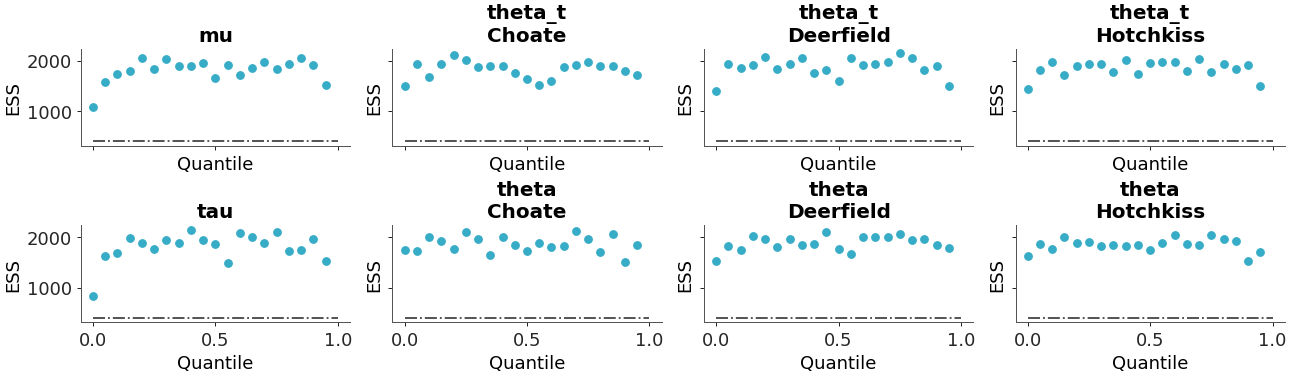
Rugs can also be added:
>>> pc = plot_ess(
>>>     non_centered,
>>>     coords={"school": ["Choate", "Deerfield", "Hotchkiss"]},
>>>     rug=True,
>>> )
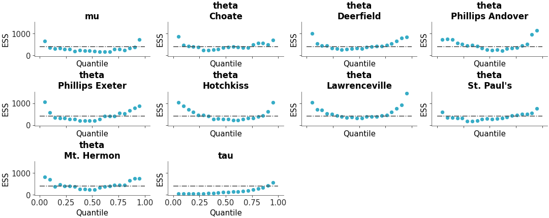
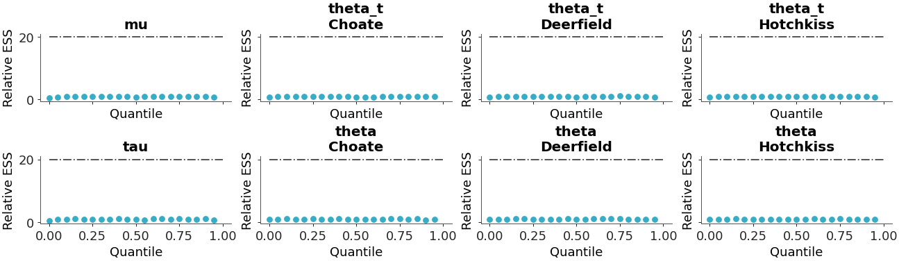
Relative ESS can be plotted instead of absolute:
>>> pc = plot_ess(
>>>     non_centered,
>>>     coords={"school": ["Choate", "Deerfield", "Hotchkiss"]},
>>>     relative=True,
>>> )
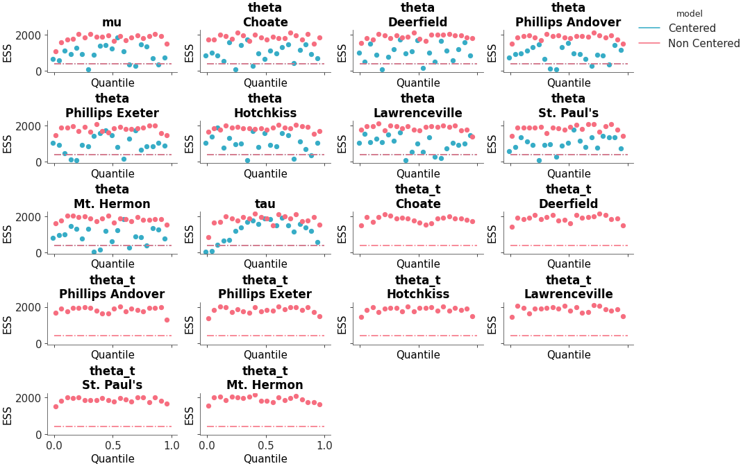
We can also adjust the number of points:
>>> pc = plot_ess(
>>>     non_centered,
>>>     coords={"school": ["Choate", "Deerfield", "Hotchkiss"]},
>>>     n_points=10,
>>> )