arviz_plots.plot_ess_evolution

arviz_plots.plot_ess_evolution(dt, var_names=None, filter_vars=None, group='posterior', coords=None, sample_dims=None, relative=False, n_points=20, extra_methods=False, min_ess=400, plot_collection=None, backend=None, labeller=None, aes_by_visuals=None, visuals=None, stats=None, **pc_kwargs)

Plot estimated effective sample size plots for increasing number of iterations.

Roughly speaking, the effective sample size of a quantity of interest captures how many independent draws contain the same amount of information as the dependent sample obtained by the MCMC algorithm. The higher the ESS the better. See [1] for more details.

Parameters:

dtxarray.DataTree or dict of {strxarray.DataTree}

Input data. In case of dictionary input, the keys are taken to be model names. In such cases, a dimension “model” is generated and can be used to map to aesthetics.

var_namesstr or sequence of str, optional

One or more variables to be plotted. Prefix the variables by ~ when you want to exclude them from the plot.

filter_vars{None, “like”, “regex”}, default None

If None, interpret var_names as the real variables names. If “like”, interpret var_names as substrings of the real variables names. If “regex”, interpret var_names as regular expressions on the real variables names.

groupstr, default “posterior”

Group to be plotted.

coordsdict, optional

sample_dimsstr or sequence of hashable, optional

Dimensions to reduce unless mapped to an aesthetic. Defaults to rcParams["data.sample_dims"]

relativebool, default False

Show relative ess in plot ress = ess / N.

n_pointsint, default 20

Number of subsets in the evolution plot.

extra_methodsbool, default False

Plot mean and sd ESS as horizontal lines.

min_essint, default 400

Minimum number of ESS desired. If relative=True the line is plotted at min_ess / n_samples as a curve following the min_ess / n dependency

plot_collectionPlotCollection, optional

backend{“matplotlib”, “bokeh”}, optional

labellerlabeller, optional

aes_by_visualsmapping of {strsequence of str or False}, optional

Mapping of visuals to aesthetics that should use their mapping in plot_collection when plotted. Valid keys are the same as for visuals.

visualsmapping of {strmapping or False}, optional

Valid keys are:

• ess_bulk -> passed to scatter_xy

• ess_bulk_line -> passed to line_xy

• ess_tail -> passed to scatter_xy

• ess_tail_line -> passed to line_xy

• title -> passed to labelled_title

• xlabel -> passed to labelled_x

• ylabel -> passed to labelled_y

• mean -> passed to line_xy

• sd -> passed to line_xy

• mean_text -> passed to annotate_xy

• sd_text -> passed to annotate_xy

• min_ess -> passed to line_xy

statsmapping, optional

Valid keys are:

• ess_bulk -> passed to ess, method = ‘bulk’

• ess_tail -> passed to ess, method = ‘tail’

• mean -> passed to ess, method=’mean’

• sd -> passed to ess, method=’sd’

**pc_kwargs

Passed to arviz_plots.PlotCollection.wrap

Returns:

PlotCollection

See also

Introduction to batteries-included plots

General introduction to batteries-included plotting functions, common use and logic overview

References

[1]

Vehtari et al. Rank-normalization, folding, and localization: An improved Rhat for assessing convergence of MCMC. Bayesian Analysis. 16(2) (2021) https://doi.org/10.1214/20-BA1221. arXiv preprint https://arxiv.org/abs/1903.08008

Examples

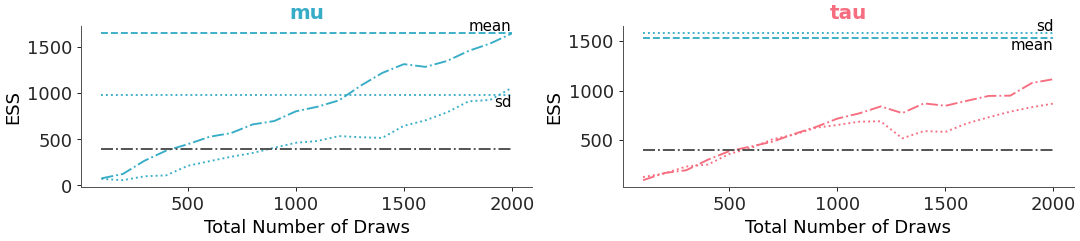
When adding a mapping for color across variables, the same color for a variable gets applied to both the ‘bulk’ and ‘tail’ ess. In such a case, if separate linestyles for ‘bulk’ and ‘tail’ are desired to distinguish them instead of colors (which is what is used by default), then this can be implemented:

>>> from arviz_plots import plot_ess_evolution, style
>>> style.use("arviz-variat")
>>> from arviz_base import load_arviz_data
>>> non_centered = load_arviz_data('non_centered_eight')
>>> pc = plot_ess_evolution(
>>>     non_centered,
>>>     var_names=["mu", "tau"],
>>>     extra_methods=True,
>>>     visuals={
>>>         "ess_bulk_line": {"linestyle": "-."},
>>>         "ess_tail_line": {"linestyle": ":"},
>>>         "ess_bulk": False,
>>>         "ess_tail": False,
>>>     },
>>>     aes= {"color": ["__variable__"]},
>>>     aes_by_visuals={"title": ["color"]},
>>> )

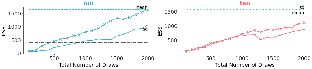
The points and lines for ess ‘bulk’ and ‘tail’ can be individually switched on and off. If only the points are desired, and a situation like the previous example occurs, markers can be used to distinguish between points for ‘bulk’ and ‘tail’:

>>> pc = plot_ess_evolution(
>>>     non_centered,
>>>     var_names=["mu", "tau"],
>>>     extra_methods=True,
>>>     visuals={
>>>         "ess_bulk": {"marker": "x"},
>>>         "ess_tail": {"marker": "_"},
>>>     },
>>>     aes={"color": ["__variable__"]},
>>>     aes_by_visuals={"title": ["color"]},
>>> )

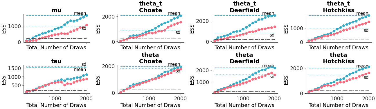
We can add extra methods to plot the mean and standard deviation as lines, and adjust the minimum ess baseline as well:

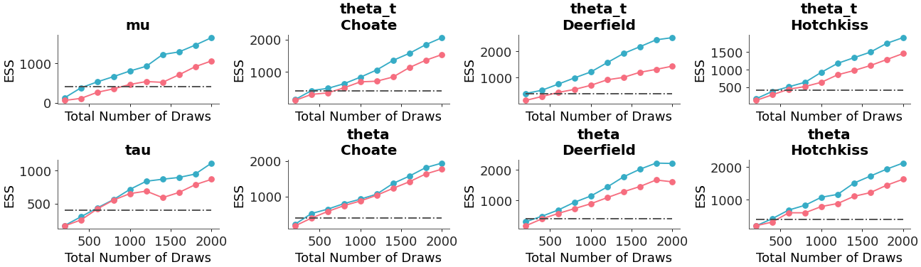
>>> pc = plot_ess_evolution(
>>>     non_centered,
>>>     coords={"school": ["Choate", "Deerfield", "Hotchkiss"]},
>>>     extra_methods=True,
>>>     min_ess=200,
>>> )

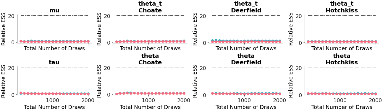
Relative ESS can be plotted instead of absolute:

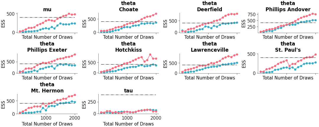
>>> pc = plot_ess_evolution(
>>>     non_centered,
>>>     coords={"school": ["Choate", "Deerfield", "Hotchkiss"]},
>>>     relative=True,
>>> )

We can also adjust the number of points:

>>> pc = plot_ess_evolution(
>>>     non_centered,
>>>     coords={"school": ["Choate", "Deerfield", "Hotchkiss"]},
>>>     n_points=10,
>>> )

faceted plot with ESS ‘bulk’ and ‘tail’ for each variable

ESS evolution

ESS evolution