arviz_plots.plot_rank_dist#
- arviz_plots.plot_rank_dist(dt, var_names=None, filter_vars=None, group='posterior', coords=None, sample_dims=None, compact=True, combined=False, kind=None, ci_prob=None, plot_collection=None, backend=None, labeller=None, aes_by_visuals=None, visuals=None, stats=None, **pc_kwargs)[source]#
Plot 1D marginal distributions and fractional rank Δ-ECDF plots.
Rank plots are built by replacing the posterior draws by their ranking computed over all chains. Then each chain is plotted independently. If all of the chains are targeting the same posterior, we expect the ranks in each chain to be uniformly distributed. To simplify comparison we compute the ordered fractional ranks, which are distributed uniformly in [0, 1]. Additionally, we plot the Δ-ECDF, that is, the difference between the expected CDF from the observed ECDF. Simultaneous confidence bands are computed using simulation method described in [1].
- Parameters:
- dt
xarray.DataTree Input data
- var_names
strorlistofstr, optional One or more variables to be plotted. Prefix the variables by ~ when you want to exclude them from the plot.
- filter_vars{
None, “like”, “regex”}, optional, default=None If None (default), interpret var_names as the real variables names. If “like”, interpret var_names as substrings of the real variables names. If “regex”, interpret var_names as regular expressions on the real variables names.
- group
str, default “posterior” Group to be plotted.
- sample_dims
stror sequence of hashable, optional Dimensions to reduce unless mapped to an aesthetic. Defaults to
rcParams["data.sample_dims"]- compactbool, default
True Plot multidimensional variables in a single plot.
- combinedbool, default
False Whether to plot intervals for each chain or not. Ignored when the “chain” dimension is not present.
- kind{“kde”, “hist”, “dot”, “ecdf”}, optional
How to represent the marginal density. Defaults to
rcParams["plot.density_kind"]- ci_prob
float, optional Indicates the probability that should be contained within the plotted credible interval for the fractional ranks. Defaults to
rcParams["stats.ci_prob"]- plot_collection
PlotCollection, optional - backend{“matplotlib”, “bokeh”}, optional
- labeller
labeller, optional - aes_by_visualsmapping, optional
Mapping of visuals to aesthetics that should use their mapping in
plot_collectionwhen plotted. The defaults depend on the combination of compact and combined, see the examples section for an illustrated description. Valid keys are the same as forvisuals.- visualsmapping of {
strmapping orFalse}, optional Valid keys are:
dist -> depending on the value of kind passed to:
“rank” -> passed to
ecdf_line“label” ->
labelled_xandlabelled_y“ticklabels” ->
ticklabel_props“xlabel_rank” ->
labelled_xremove_axis -> not passed anywhere, can only be
Falseto skip calling this function
- statsmapping, optional
Valid keys are:
dist -> passed to kde, ecdf, …
ecdf_pit -> passed to
ecdf_pit. Default is{"n_simulation": 1000}.
- **pc_kwargs
Passed to
arviz_plots.PlotCollection.grid
- dt
- Returns:
References
[1]Säilynoja et al. Graphical test for discrete uniformity and its applications in goodness-of-fit evaluation and multiple sample comparison. Statistics and Computing 32(32). (2022) https://doi.org/10.1007/s11222-022-10090-6
Examples
The following examples focus on behaviour specific to
plot_rank_dist. For a general introduction to batteries-included functions like this one and common usage examples see Introduction to batteries-included plotsDefault plot_rank_dist (
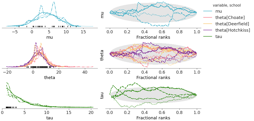
compact=Trueandcombined=False). In this case, the multiple coordinate values are overlaid on the same plot for multidimensional values; by default, the color is mapped to all dimensions of each variable (but sample_dims) to allow distinguishing the different coordinate values.As
combined=Falseeach chain is also being plotted, overlaying them on their corresponding plots; as the color property is already taken, the chain information is encoded in the linestyle as default.Both mappings are applied to the rank and dist elements.
>>> from arviz_plots import plot_rank_dist, style
>>> style.use("arviz-variat")
>>> from arviz_base import load_arviz_data
>>> centered = load_arviz_data('centered_eight')
>>> coords = {"school": ["Choate", "Deerfield", "Hotchkiss"]}
>>> pc = plot_rank_dist(centered, coords=coords, compact=True, combined=False)
>>> pc.add_legend(["__variable__", "school"])
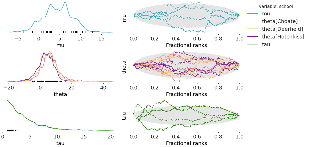
plot_rank_dist with
compact=Trueandcombined=True. The aesthetic mappings stay the same as in the previous case, but now the linestyle property mapping is only taken into account for the rank as in the left column, we use the data from all chains to generate a single distribution representation for each variable+coordinate value combination.Similarly to the first case, this default and now only mapping is applied to both the rank and the dist elements.
>>> pc = plot_rank_dist(centered, coords=coords, compact=True, combined=True)
>>> pc.add_legend(["__variable__", "school"])
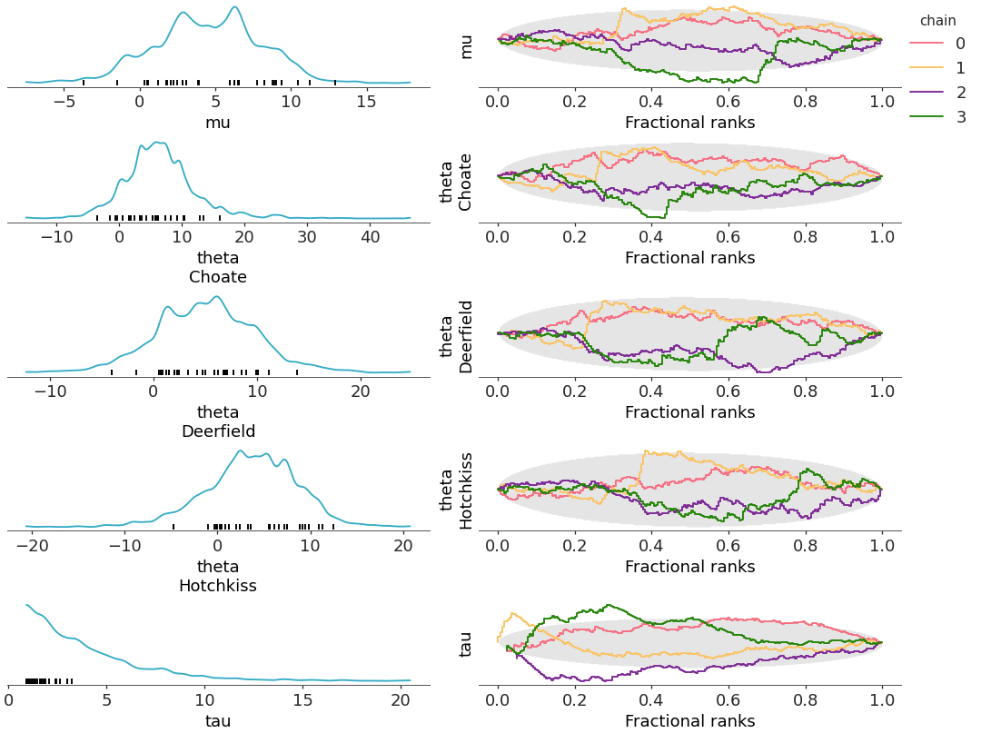
When
compact=False, each variable and coordinate value gets its own plot, and so the color property is no longer used to encode this information. Instead, it is now used to encode the chain information.>>> pc = plot_rank_dist(centered, coords=coords, compact=False, combined=False)
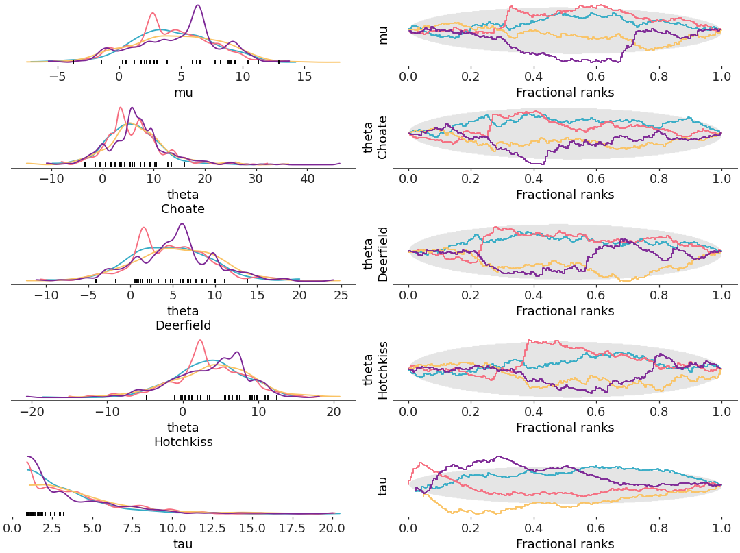
Similarly to the other
combined=Truecase, the aesthetics stay the same as withcombined=False, but they are ignored by default when plotting on the left column.>>> pc = plot_rank_dist(centered, coords=coords, compact=False, combined=True) >>> pc.add_legend("chain")