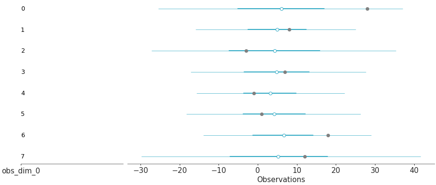
arviz_plots.plot_forest#
- arviz_plots.plot_forest(dt, var_names=None, filter_vars=None, group='posterior', coords=None, sample_dims=None, combined=False, point_estimate=None, ci_kind=None, ci_probs=None, labels=None, shade_label=None, plot_collection=None, backend=None, labeller=None, aes_by_visuals=None, visuals=None, stats=None, **pc_kwargs)[source]#
Plot 1D marginal credible intervals in a single plot.
- Parameters:
- dt
xarray.DataTreeordictof {strxarray.DataTree} Input data. In case of dictionary input, the keys are taken to be model names. In such cases, a dimension “model” is generated and can be used to map to aesthetics.
plot_forestuses the dimension “column” (creating it if necessary) to generate the grid then adds the intervals+point estimates to its “forest” coordinate and labels to its “labels” coordinates. The data used to plot is then the subsetcolumn="forest".- var_names
strorlistofstr, optional One or more variables to be plotted. Prefix the variables by ~ when you want to exclude them from the plot.
- filter_vars{
None, “like”, “regex”}, defaultNone If None, interpret var_names as the real variables names. If “like”, interpret var_names as substrings of the real variables names. If “regex”, interpret var_names as regular expressions on the real variables names.
- group
str, default “posterior” Group to be plotted.
- coords
dict, optional - sample_dims
stror sequence of hashable, optional Dimensions to reduce unless mapped to an aesthetic. Defaults to
rcParams["data.sample_dims"]- combinedbool, default
False Whether to plot intervals for each chain or not. Ignored when the “chain” dimension is not present.
- point_estimate{“mean”, “median”, “mode”}, optional
Which point estimate to plot. Defaults to rcParam
stats.point_estimate- ci_kind{“eti”, “hdi”}, optional
Which credible interval to use. Defaults to
rcParams["stats.ci_kind"]- ci_probs(
float,float), optional Indicates the probabilities that should be contained within the plotted credible intervals. It should be sorted as the elements refer to the probabilities of the “trunk” and “twig” elements. Defaults to
(0.5, rcParams["stats.ci_prob"])- labelssequence of
str, optional Sequence with the dimensions to be labelled in the plot. By default all dimensions except “chain” and “model” (if present). The order of labels is ignored, only elements being present in it matters. It can include the special “__variable__” indicator, and does so by default.
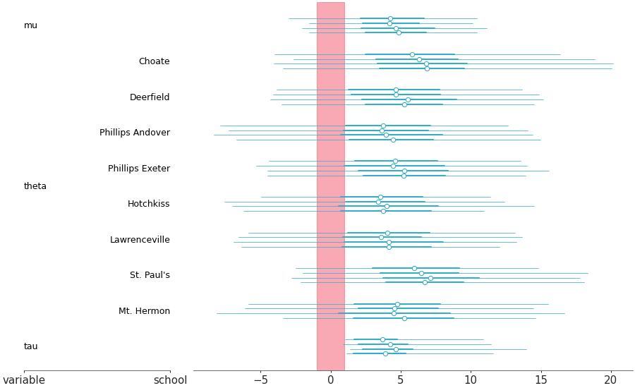
- shade_label
str, defaultNone Element of labels that should be used to add shading horizontal strips to the plot. Note that labels and credible intervals are plotted in different plots. The shading is applied to both plots, and the spacing between them is set to 0 if possible, which is not always the case (one notable example being matplotlib’s constrained layout).
- plot_collection
PlotCollection, optional - backend{“matplotlib”, “bokeh”}, optional
- labeller
labeller, optional - aes_by_visualsmapping of {
strsequence ofstrorFalse}, optional Mapping of visuals to aesthetics that should use their mapping in
plot_collectionwhen plotted. Valid keys are the same as forvisualsexcept “ticklabels” and “remove_axis” which do not apply, and “twig” and “trunk” which take the same aesthetics through the “credible_interval” key.By default, aesthetic mappings are generated for: y, alpha, overlay and color (if multiple models are present). All aesthetic mappings but alpha are applied to both the credible intervals and the point estimate; overlay is applied to labels; and both overlay and alpha are applied to the shade.
“overlay” is a dummy aesthetic to trigger looping over variables and/or dimensions using all aesthetics in every iteration. “alpha” gets two values (0, 0.3) in order to trigger the alternate shading effect.
- visualsmapping of {
strmapping orFalse}, optional Valid keys are:
trunk, twig -> passed to
line_xpoint_estimate -> passed to
scatter_xlabels -> passed to
annotate_labelshade -> passed to
fill_between_yticklabels -> passed to
xticksremove_axis -> not passed anywhere, can only take
Falseas value to skip callingremove_axis
- statsmapping, optional
Valid keys are:
trunk, twig -> passed to eti or hdi
point_estimate -> passed to mean, median or mode
- **pc_kwargs
Passed to
arviz_plots.PlotCollection.grid
- dt
- Returns:
See also
- Introduction to batteries-included plots
General introduction to batteries-included plotting functions, common use and logic overview
plot_ridgeVisual representation of marginal distributions over the y axis
Notes
The separation between variables and all its coordinate values is set to 1. The only two exceptions to this are the dimensions named “chain” and “model” in case they are present, which get a smaller spacing to give a sense of grouping among visual elements that only differ on their chain or model id.
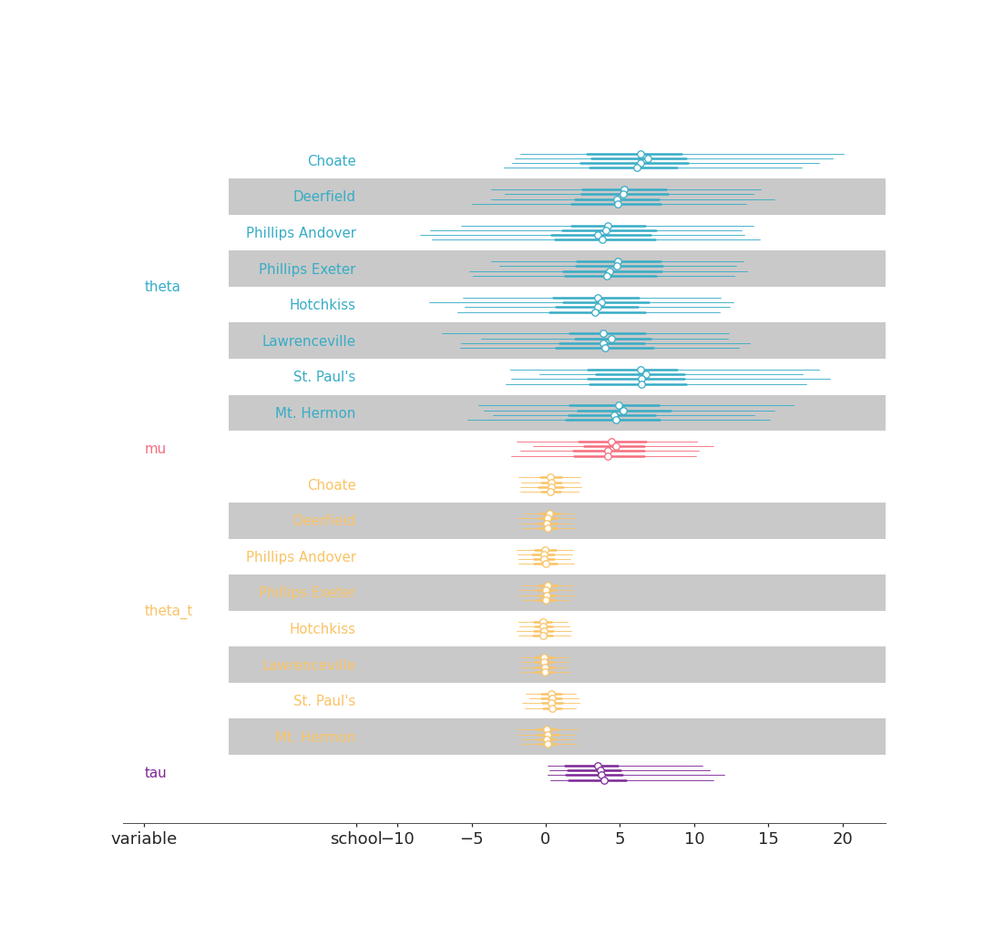
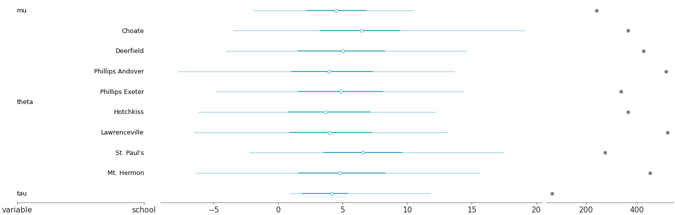
Examples
Single model forest plot with color mapped to the variable (mapping which is also applied to the labels) and alternate shading per school. Moreover, to ensure the shading looks continuous, we’ll specify we don’t want to use constrained layout (set by the “arviz-variat” theme) and to avoid having the labels too squished we’ll set the
width_ratiosforcreate_plotting_gridviapc_kwargs.>>> from arviz_plots import plot_forest, style >>> style.use("arviz-variat") >>> from arviz_base import load_arviz_data >>> non_centered = load_arviz_data('non_centered_eight') >>> pc = plot_forest( >>> non_centered, >>> var_names=["theta", "mu", "theta_t", "tau"], >>> aes={"color": ["__variable__"]}, >>> figure_kwargs={"width_ratios": [1, 2], "layout": "none"}, >>> aes_by_visuals={"labels": ["color"]}, >>> shade_label="school", >>> )