arviz_plots.plot_ppc_tstat#
- arviz_plots.plot_ppc_tstat(dt, var_names=None, group='posterior_predictive', filter_vars=None, sample_dims=None, t_stat='median', kind=None, point_estimate=None, ci_kind=None, ci_prob=None, plot_collection=None, coords=None, backend=None, data_pairs=None, labeller=None, aes_by_visuals=None, visuals=None, stats=None, **pc_kwargs)[source]#
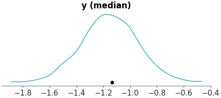
Plot Bayesian t-stat for observed data and posterior/prior predictive.
- Parameters:
- dt
xarray.DataTree If group is “posterior_predictive”, it should contain the
posterior_predictiveandobserved_datagroups. If group is “prior_predictive”, it should contain theprior_predictivegroup.- var_names
strorlistofstr, optional One or more variables to be plotted. Prefix the variables by ~ when you want to exclude them from the plot.
- groupstr,
Group to be plotted. Defaults to “posterior_predictive”. It could also be “prior_predictive”.
- filter_vars{
None, “like”, “regex”}, default=None If None, interpret var_names as the real variables names. If “like”, interpret var_names as substrings of the real variables names. If “regex”, interpret var_names as regular expressions on the real variables names.
- sample_dims
stror sequence of hashable, optional Dimensions to reduce unless mapped to an aesthetic. Defaults to
rcParams["data.sample_dims"]- t_stat
str,float, orcallable() default “median” Test statistics to compute from the observations and predictive distributions. Allowed strings are “mean”, “median”, “std”, “var”, “min”, “max”, “iqr” (interquartile range) and “mad” (median absolute deviation). Alternative a quantile can be passed as a float (or str) in the interval (0, 1). Finally, a user defined function is also accepted.
- kind{“kde”, “hist”, “dot”, “ecdf”}, optional
How to represent the marginal density. Defaults to
rcParams["plot.density_kind"]- point_estimate{“mean”, “median”, “mode”}, optional
Which point estimate to plot. Defaults to rcParam
stats.point_estimate- ci_kind{“eti”, “hdi”}, optional
Which credible interval to use. Defaults to
rcParams["stats.ci_kind"]- ci_prob
float, optional Indicates the probability that should be contained within the plotted credible interval. Defaults to
rcParams["stats.ci_prob"]- plot_collection
PlotCollection, optional - coords
dict, optional - backend{“matplotlib”, “bokeh”, “plotly”}, optional
- labeller
labeller, optional - data_pairs
dict, optional Dictionary of keys prior/posterior predictive data and values observed data variable names. If None, it will assume that the observed data and the predictive data have the same variable name.
- aes_by_visualsmapping of {
strsequence ofstr}, optional Mapping of visuals to aesthetics that should use their mapping in
plot_collectionwhen plotted. Valid keys are the same as forvisualsexept for “remove_axis”- visualsmapping of {
strmapping orFalse}, optional Valid keys are:
dist -> depending on the value of kind passed to:
observed_tstat -> passed to
scatter_x.credible_interval -> passed to
line_x. Defaults to False.point_estimate -> passed to
scatter_x. Defaults to False.point_estimate_text -> passed to
point_estimate_text. Defaults to False.title -> passed to
labelled_titlerug -> passed to
scatter_x. Defaults to False.remove_axis -> not passed anywhere, can only be
Falseto skip calling this function
observed_tstat defaults to False, no observed data is plotted, if group is “prior_predictive”. Pass an (empty) mapping to plot the observed tstats.
- statsmapping, optional
Valid keys are:
dist -> passed to kde, ecdf, …
- **pc_kwargs
Passed to
arviz_plots.PlotCollection.wrap
- dt
- Returns:
Examples
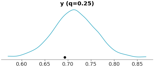
Use 25th percentile (quantile 0.25) as t-statistic
>>> from arviz_plots import plot_ppc_tstat, style
>>> style.use("arviz-variat")
>>> from arviz_base import load_arviz_data
>>> dt = load_arviz_data('radon')
>>> plot_ppc_tstat(dt, t_stat="0.25")
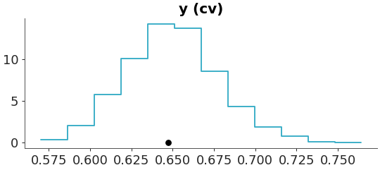
Define custom t-statistic function and plot histogram
>>> def cv(x):
>>>     return np.std(x, axis=0) / np.mean(x, axis=0)
>>> plot_ppc_tstat(dt, t_stat=cv, kind="hist")
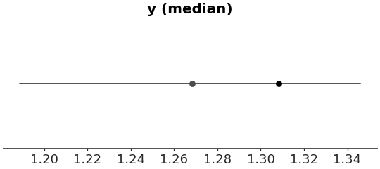
Use median as t-statistic and plot point-interval
>>> azp.plot_ppc_tstat(
>>>     dt,
>>>     visuals={
>>>         "dist": False,
>>>         "credible_interval": {},
>>>         "point_estimate": {},
>>>     }
>>> )