arviz_plots.plot_ppc_pit#
- arviz_plots.plot_ppc_pit(dt, ci_prob=None, coverage=False, var_names=None, data_pairs=None, filter_vars=None, group='posterior_predictive', coords=None, sample_dims=None, plot_collection=None, backend=None, labeller=None, aes_by_visuals=None, visuals=None, stats=None, **pc_kwargs)[source]#
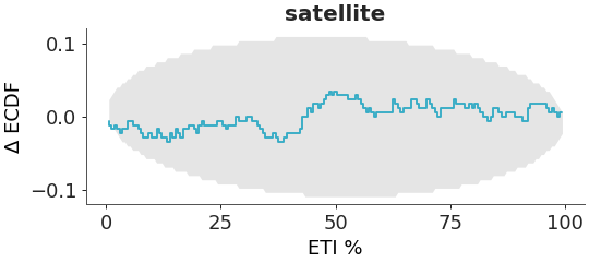
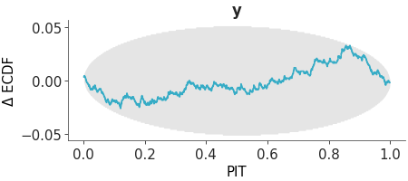
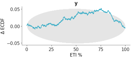
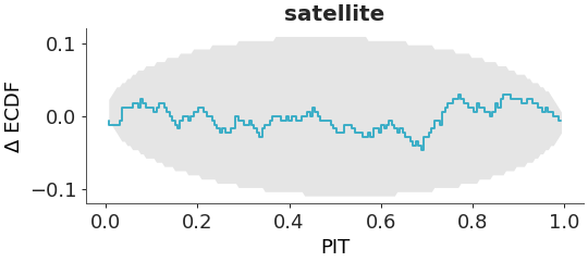
PIT Δ-ECDF values with simultaneous confidence envelope.
For a calibrated model the Probability Integral Transform (PIT) values, $p(tilde{y}_i le y_i mid y)$, should be uniformly distributed. Where $y_i$ represents the observed data for index $i$ and $tilde y_i$ represents the posterior predictive sample at index $i$.
This plot shows the empirical cumulative distribution function (ECDF) of the PIT values. To make the plot easier to interpret, we plot the Δ-ECDF, that is, the difference between the observed ECDF and the expected CDF. Simultaneous confidence bands are computed using the method described in described in [1].
Alternatively, we can visualize the coverage of the central posterior credible intervals by setting
coverage=True. This allows us to assess whether the credible intervals includes the observed values. We can obtain the coverage of the central intervals from the PIT by replacing the PIT with two times the absolute difference between the PIT values and 0.5.For more details on how to interpret this plot, see https://arviz-devs.github.io/EABM/Chapters/Prior_posterior_predictive_checks.html#pit-ecdfs.
- Parameters:
- dt
xarray.DataTree Input data
- ci_prob
float, optional Indicates the probability that should be contained within the plotted credible interval. Defaults to
rcParams["stats.ci_prob"]- coveragebool, optional
If True, plot the coverage of the central posterior credible intervals. Defaults to False.
- data_pairs
dict, optional Dictionary of keys prior/posterior predictive data and values observed data variable names. If None, it will assume that the observed data and the predictive data have the same variable name.
- var_names
strorlistofstr, optional One or more variables to be plotted. Currently only one variable is supported. Prefix the variables by ~ when you want to exclude them from the plot.
- filter_vars{
None, “like”, “regex”}, optional, default=None If None (default), interpret var_names as the real variables names. If “like”, interpret var_names as substrings of the real variables names. If “regex”, interpret var_names as regular expressions on the real variables names.
- groupstr,
Group to be plotted. Defaults to “posterior_predictive”. It could also be “prior_predictive”.
- coords
dict, optional Coordinates to plot.
- sample_dims
stror sequence of hashable, optional Dimensions to reduce unless mapped to an aesthetic. Defaults to
rcParams["data.sample_dims"]- plot_collection
PlotCollection, optional - backend{“matplotlib”, “bokeh”, “plotly”}, optional
- labeller
labeller, optional - aes_by_visualsmapping of {
strsequence ofstr}, optional Mapping of visuals to aesthetics that should use their mapping in
plot_collectionwhen plotted. Valid keys are the same as forvisuals.- visualsmapping of {
strmapping orFalse}, optional Valid keys are:
ecdf_lines -> passed to
ecdf_lineci -> passed to
ci_line_yxlabel -> passed to
labelled_xylabel -> passed to
labelled_ytitle -> passed to
labelled_title
- statsmapping, optional
Valid keys are:
ecdf_pit -> passed to
ecdf_pit. Default is{"n_simulation": 1000}.
- **pc_kwargs
Passed to
arviz_plots.PlotCollection.wrap
- dt
- Returns:
References
[1]Säilynoja et al. Graphical test for discrete uniformity and its applications in goodness-of-fit evaluation and multiple sample comparison. Statistics and Computing 32(32). (2022) https://doi.org/10.1007/s11222-022-10090-6
Examples
Plot the ecdf-PIT for the crabs hurdle-negative-binomial dataset.
>>> from arviz_plots import plot_ppc_pit, style
>>> style.use("arviz-variat")
>>> from arviz_base import load_arviz_data
>>> dt = load_arviz_data('crabs_hurdle_nb')
>>> plot_ppc_pit(dt)
Plot the coverage for the crabs hurdle-negative-binomial dataset.
>>> plot_ppc_pit(dt, coverage=True)